Tutorial: Solution of the linear advection equation

This tutorial is about the efficient solution of production-destruction systems (PDS) with a large number of differential equations. We will explore several ways to represent such large systems and assess their efficiency.

Definition of the production-destruction system

One example of the occurrence of a PDS with a large number of equations is the space discretization of a partial differential equation. In this tutorial we want to solve the linear advection equation

\[\partial_t u(t,x)=-a\partial_x u(t,x),\quad u(0,x)=u_0(x)\]

with $a>0$, $t≥ 0$, $x\in[0,1]$ and periodic boundary conditions. To keep things as simple as possible, we discretize the space domain as $0=x_0<x_1\dots <x_{N-1}<x_N=1$ with $x_i = i Δ x$ for $i=0,\dots,N$ and $Δx=1/N$. An upwind discretization of the spatial derivative yields the ODE system

\[\begin{aligned} &\partial_t u_1(t) =-\frac{a}{Δx}\bigl(u_1(t)-u_{N}(t)\bigr),\\ &\partial_t u_i(t) =-\frac{a}{Δx}\bigl(u_i(t)-u_{i-1}(t)\bigr),\quad i=2,\dots,N, \end{aligned}\]

where $u_i(t)$ is an approximation of $u(t,x_i)$ for $i=1,\dots, N$. This system can also be written as $\partial_t \mathbf u(t)=\mathbf A\mathbf u(t)$ with $\mathbf u(t)=(u_1(t),\dots,u_N(t))$ and

\[\mathbf A= \frac{a}{Δ x}\begin{bmatrix}-1&0&\dots&0&1\\1&-1&\ddots&&0\\0&\ddots&\ddots&\ddots&\vdots\\ \vdots&\ddots&\ddots&\ddots&0\\0&\dots&0&1&-1\end{bmatrix}.\]

In particular the matrix $\mathbf A$ shows that there is a single production term and a single destruction term per equation. Furthermore, the system is conservative as $\mathbf A$ has column sum zero. To be precise, the production matrix $\mathbf P = (p_{i,j})$ of this conservative PDS is given by

\[\begin{aligned} &p_{1,N}(t,\mathbf u(t)) = \frac{a}{Δ x}u_N(t),\\ &p_{i,i-1}(t,\mathbf u(t)) = \frac{a}{Δ x}u_{i-1}(t),\quad i=2,\dots,N. \end{aligned}\]

In addition, all production and destruction terms not listed have the value zero. Since the PDS is conservative, we have $d_{i,j}=p_{j,i}$ and the system is fully determined by the production matrix $\mathbf P$.

Solution of the production-destruction system

Now we are ready to define a ConservativePDSProblem and to solve this problem with a method of PositiveIntegrators.jl or OrdinaryDiffEq.jl. In the following we use $a=1$, $N=1000$ and the time domain $t\in[0,1]$. Moreover, we choose the step function

\[u_0(x)=\begin{cases}1, & 0.4 ≤ x ≤ 0.6,\\ 0,& \text{elsewhere}\end{cases}\]

as initial condition. Due to the periodic boundary conditions and the transport velocity $a=1$, the solution at time $t=1$ is identical to the initial distribution, i.e. $u(1,x) = u_0(x)$.

N = 1000 # number of subintervalsdx = 1/N # mesh widthx = LinRange(dx, 1.0, N) # discretization points x_1,...,x_N = x_0u0 = @. 0.0 + (0.4 ≤ x ≤ 0.6) * 1.0 # initial solutiontspan = (0.0, 1.0) # time domain

As mentioned above, we will try different approaches to solve this PDS and compare their efficiency. These are

an in-place implementation with a dense matrix,
an in-place implementation with a sparse matrix.

Standard in-place implementation

By default, we will use dense matrices to store the production terms and to setup/solve the linear systems arising in MPRK methods. Of course, this is not efficient for large and sparse systems like in this case.

using PositiveIntegrators # load ConservativePDSProblemfunction lin_adv_P!(P, u, p, t)    fill!(P, 0.0)    N = length(u)    dx = 1 / N    P[1, N] = u[N] / dx    for i in 2:N        P[i, i - 1] = u[i - 1] / dx    end    return nothingendprob = ConservativePDSProblem(lin_adv_P!, u0, tspan) # create the PDSsol = solve(prob, MPRK43I(1.0, 0.5); save_everystep = false)

using Plotsplot(x, u0; label = "u0", xguide = "x", yguide = "u")plot!(x, last(sol.u); label = "u")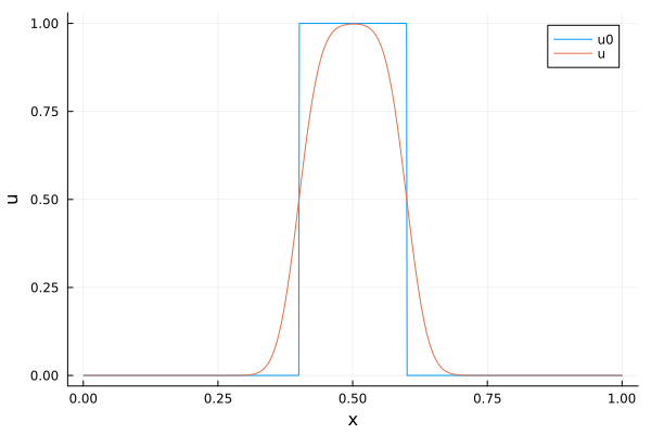

We can use isnonnegative to check that the computed solution is nonnegative, as expected from an MPRK scheme.

isnonnegative(sol)

true

Using sparse matrices

To use different matrix types for the production terms and linear systems, we can use the keyword argument p_prototype of ConservativePDSProblem and PDSProblem.

using SparseArraysp_prototype = spdiagm(-1 => ones(eltype(u0), N - 1),                      N - 1 => ones(eltype(u0), 1))prob_sparse = ConservativePDSProblem(lin_adv_P!, u0, tspan; p_prototype=p_prototype)sol_sparse = solve(prob_sparse, MPRK43I(1.0, 0.5); save_everystep = false)

plot(x,u0; label = "u0", xguide = "x", yguide = "u")plot!(x, last(sol_sparse.u); label = "u")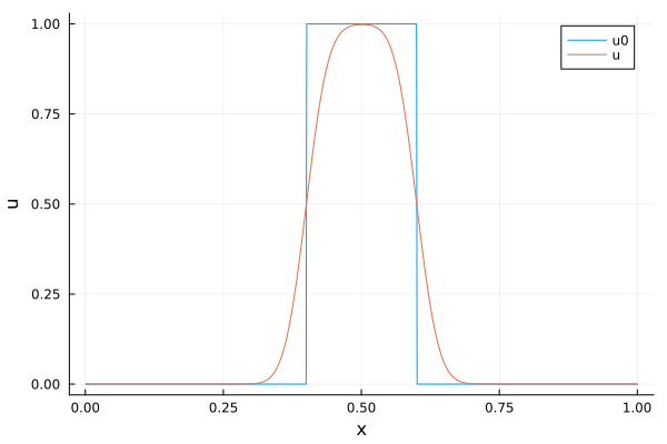

Also this solution is nonnegative.

isnonnegative(sol_sparse)

true

Performance comparison

Finally, we use BenchmarkTools.jl to compare the performance of the different implementations.

using BenchmarkTools@benchmark solve(prob, MPRK43I(1.0, 0.5); save_everystep = false)

BenchmarkTools.Trial: 1 sample with 1 evaluation per sample.
 Single result which took 34.287 s (0.00% GC) to evaluate,
 with a memory estimate of 23.01 MiB, over 86 allocations.

@benchmark solve(prob_sparse, MPRK43I(1.0, 0.5); save_everystep = false)

BenchmarkTools.Trial: 4 samples with 1 evaluation per sample.
 Range (min … max):  1.331 s …   1.372 s  ┊ GC (min … max): 4.88% … 5.42%
 Time  (median):     1.343 s              ┊ GC (median):    4.84%
 Time  (mean ± σ):   1.347 s ± 19.045 ms  ┊ GC (mean ± σ):  4.96% ± 0.31%

  █   █                      █                            █  
  █▁▁▁█▁▁▁▁▁▁▁▁▁▁▁▁▁▁▁▁▁▁▁▁▁▁█▁▁▁▁▁▁▁▁▁▁▁▁▁▁▁▁▁▁▁▁▁▁▁▁▁▁▁▁█ ▁
  1.33 s         Histogram: frequency by time        1.37 s <

 Memory estimate: 1.69 GiB, allocs estimate: 86780.

By default, we use an LU factorization for the linear systems. At the time of writing, Julia uses SparseArrays.jl defaulting to UMFPACK from SuiteSparse in this case. However, the linear systems do not necessarily have the structure for which UMFPACK is optimized for. Thus, it is often possible to gain performance by switching to KLU instead.

using LinearSolve@benchmark solve(prob_sparse, MPRK43I(1.0, 0.5; linsolve = KLUFactorization()); save_everystep = false)

BenchmarkTools.Trial: 26 samples with 1 evaluation per sample.
 Range (min … max):  182.825 ms … 218.447 ms  ┊ GC (min … max): 0.00% … 0.00%
 Time  (median):     191.386 ms               ┊ GC (median):    0.00%
 Time  (mean ± σ):   192.331 ms ±   7.748 ms  ┊ GC (mean ± σ):  0.00% ± 0.00%

  ▁█ ▁▁▁ █   ▁▁███  ▁▁█ ▁▁  █                ▁                ▁  
  ██▁███▁█▁▁▁█████▁▁███▁██▁▁█▁▁▁▁▁▁▁▁▁▁▁▁▁▁▁▁█▁▁▁▁▁▁▁▁▁▁▁▁▁▁▁▁█ ▁
  183 ms           Histogram: frequency by time          218 ms <

 Memory estimate: 1.07 MiB, allocs estimate: 277.

Package versions

These results were obtained using the following versions.

using InteractiveUtilsversioninfo()println()using PkgPkg.status(["PositiveIntegrators", "SparseArrays", "KLU", "LinearSolve"],           mode=PKGMODE_MANIFEST)

Julia Version 1.13.1
Commit 96ca370cf0e (2026-09-25 19:34 UTC)
Build Info:
  Official https://julialang.org release
Platform Info:
  OS: Linux (x86_64-linux-gnu)
  CPU: 4 × AMD EPYC 7763 64-Core Processor
  WORD_SIZE: 64
  LLVM: libLLVM-20.1.8 (ORCJIT, znver3)
  GC: Built with stock GC
Threads: 1 default, 1 interactive, 1 GC (on 4 virtual cores)
Environment:
  JULIA_PKG_SERVER_REGISTRY_PREFERENCE = eager

Status `~/work/PositiveIntegrators.jl/PositiveIntegrators.jl/docs/Manifest.toml`
  [14f7f29c] AMD v0.5.4
  [4fba245c] ArrayInterface v7.30.2
  [2569d6c7] ConcreteStructs v0.2.8
  [ffbed154] DocStringExtensions v0.9.5
  [4e289a0a] EnumX v1.0.7
  [7034ab61] FastBroadcast v1.4.0
  [46192b85] GPUArraysCore v0.2.1
  [ba0b0d4f] Krylov v0.10.10
  [2faa5264] LHLFactorization v2.2.2
  [7ed4a6bd] LinearSolve v5.18.2
  [46d2c3a1] MuladdMacro v0.2.7
  [bbf590c4] OrdinaryDiffEqCore v4.18.1
  [d1b20bf0] PositiveIntegrators v0.2.22-DEV `~/work/PositiveIntegrators.jl/PositiveIntegrators.jl`
  [d236fae5] PreallocationTools v1.7.1
  [aea7be01] PrecompileTools v1.3.4
  [21216c6a] Preferences v1.6.0
  [0c0d3e7f] PureKLU v1.6.0
  [3cdcf5f2] RecipesBase v1.4.0
  [731186ca] RecursiveArrayTools v4.5.3
  [189a3867] Reexport v1.2.2
  [0bca4576] SciMLBase v3.57.0
  [a6db7da4] SciMLLogging v2.1.0
  [c0aeaf25] SciMLOperators v1.30.2
  [53ae85a6] SciMLStructures v1.10.5
  [efcf1570] Setfield v1.1.2
  [a57abbd0] SparseColumnPivotedQR v2.1.8
  [90137ffa] StaticArrays v1.9.22
  [1e83bf80] StaticArraysCore v1.4.4
  [10745b16] Statistics v1.11.5
  [2efcf032] SymbolicIndexingInterface v0.3.55
  [856f044c] MKL_jll v2025.2.0+0
  [b77e0a4c] InteractiveUtils v1.11.0
  [8f399da3] Libdl v1.11.0
  [37e2e46d] LinearAlgebra v1.13.0
  [d6f4376e] Markdown v1.11.0
  [9a3f8284] Random v1.11.0
  [9e88b42a] Serialization v1.11.0
  [2f01184e] SparseArrays v1.13.0
  [4536629a] OpenBLAS_jll v0.3.30+0
  [bea87d4a] SuiteSparse_jll v7.10.1+0