Tutorial: Solution of the heat equation with Dirichlet boundary conditions

We continue the previous tutorial on solving the heat equation with Neumann boundary conditions by looking at Dirichlet boundary conditions instead, resulting in a non-conservative production-destruction system.

Definition of the (non-conservative) production-destruction system

Consider the heat equation

\[\partial_t u(t,x) = \mu \partial_x^2 u(t,x),\quad u(0,x)=u_0(x),\]

with $μ ≥ 0$, $t≥ 0$, $x\in[0,1]$, and homogeneous Dirichlet boundary conditions. We use again a finite volume discretization, i.e., we split the domain $[0, 1]$ into $N$ uniform cells of width $\Delta x = 1 / N$. As degrees of freedom, we use the mean values of $u(t)$ in each cell approximated by the point value $u_i(t)$ in the center of cell $i$. Finally, we use the classical central finite difference discretization of the Laplacian with homogeneous Dirichlet boundary conditions, resulting in the ODE

\[\partial_t u(t) = L u(t), \quad L = \frac{\mu}{\Delta x^2} \begin{pmatrix} -2 & 1 \\ 1 & -2 & 1 \\ & \ddots & \ddots & \ddots \\ && 1 & -2 & 1 \\ &&& 1 & -2 \end{pmatrix}.\]

The system can be written as a non-conservative PDS with production terms

\[\begin{aligned} &p_{i,i-1}(t,\mathbf u(t)) = \frac{\mu}{\Delta x^2} u_{i-1}(t),\quad i=2,\dots,N, \\ &p_{i,i+1}(t,\mathbf u(t)) = \frac{\mu}{\Delta x^2} u_{i+1}(t),\quad i=1,\dots,N-1, \end{aligned}\]

and destruction terms $d_{i,j} = p_{j,i}$ for $i \ne j$ as well as the non-conservative destruction terms

\[\begin{aligned} d_{1,1}(t,\mathbf u(t)) &= \frac{\mu}{\Delta x^2} u_{1}(t), \\ d_{N,N}(t,\mathbf u(t)) &= \frac{\mu}{\Delta x^2} u_{N}(t). \end{aligned}\]

In addition, all production and destruction terms not listed are zero.

Solution of the non-conservative production-destruction system

Now we are ready to define a PDSProblem and to solve this problem with a method of PositiveIntegrators.jl or OrdinaryDiffEq.jl. In the following we use $N = 100$ nodes and the time domain $t \in [0,1]$. Moreover, we choose the initial condition

\[u_0(x) = \sin(\pi x)^2.\]

x_boundaries = range(0, 1, length = 101)x = x_boundaries[1:end-1] .+ step(x_boundaries) / 2u0 = @. sinpi(x)^2 # initial solutiontspan = (0.0, 1.0) # time domain

We will choose three different matrix types for the production terms and the resulting linear systems:

standard dense matrices (default)
sparse matrices (from SparseArrays.jl)
tridiagonal matrices (from LinearAlgebra.jl)

Standard dense matrices

using PositiveIntegrators # load ConservativePDSProblemfunction heat_eq_P!(P, u, μ, t)    fill!(P, 0)    N = length(u)    Δx = 1 / N    μ_Δx2 = μ / Δx^2    let i = 1        # Dirichlet boundary condition        P[i, i + 1] = u[i + 1] * μ_Δx2    end    for i in 2:(length(u) - 1)        # interior stencil        P[i, i - 1] = u[i - 1] * μ_Δx2        P[i, i + 1] = u[i + 1] * μ_Δx2    end    let i = length(u)        # Dirichlet boundary condition        P[i, i - 1] = u[i - 1] * μ_Δx2    end    return nothingendfunction heat_eq_D!(D, u, μ, t)    fill!(D, 0)    N = length(u)    Δx = 1 / N    μ_Δx2 = μ / Δx^2    # Dirichlet boundary condition    D[begin] = u[begin] * μ_Δx2    D[end] = u[end] * μ_Δx2    return nothingendμ = 1.0e-2prob = PDSProblem(heat_eq_P!, heat_eq_D!, u0, tspan, μ) # create the PDSsol = solve(prob, MPRK22(1.0); save_everystep = false)

using Plotsplot(x, u0; label = "u0", xguide = "x", yguide = "u")plot!(x, last(sol.u); label = "u")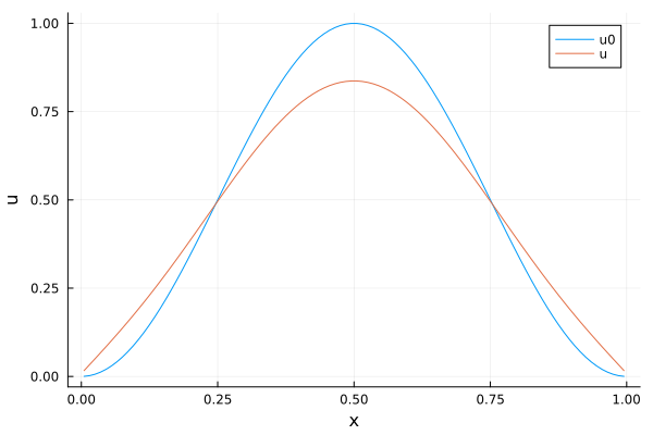

Sparse matrices

To use different matrix types for the production terms and linear systems, you can use the keyword argument p_prototype of ConservativePDSProblem and PDSProblem.

using SparseArraysp_prototype = spdiagm(-1 => ones(eltype(u0), length(u0) - 1),                      +1 => ones(eltype(u0), length(u0) - 1))prob_sparse = PDSProblem(heat_eq_P!, heat_eq_D!, u0, tspan, μ;                         p_prototype = p_prototype)sol_sparse = solve(prob_sparse, MPRK22(1.0); save_everystep = false)

plot(x, u0; label = "u0", xguide = "x", yguide = "u")plot!(x, last(sol_sparse.u); label = "u")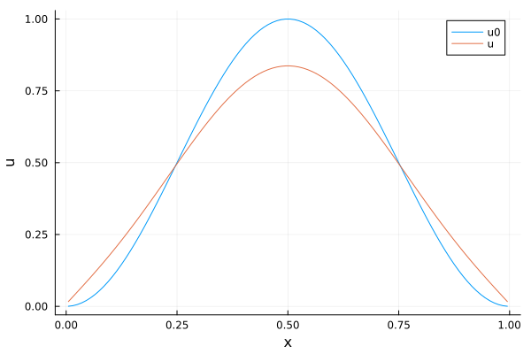

Tridiagonal matrices

The sparse matrices used in this case have a very special structure since they are in fact tridiagonal matrices. Thus, we can also use the special matrix type Tridiagonal from the standard library LinearAlgebra.

using LinearAlgebrap_prototype = Tridiagonal(ones(eltype(u0), length(u0) - 1),                          ones(eltype(u0), length(u0)),                          ones(eltype(u0), length(u0) - 1))prob_tridiagonal = PDSProblem(heat_eq_P!, heat_eq_D!, u0, tspan, μ;                              p_prototype = p_prototype)sol_tridiagonal = solve(prob_tridiagonal, MPRK22(1.0); save_everystep = false)

plot(x, u0; label = "u0", xguide = "x", yguide = "u")plot!(x, last(sol_tridiagonal.u); label = "u")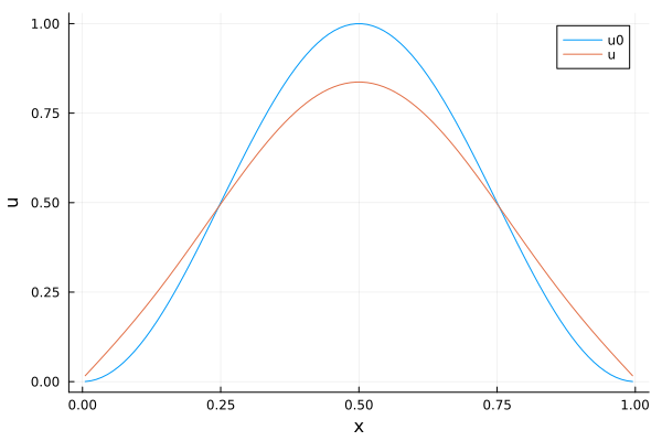

Performance comparison

Finally, we use BenchmarkTools.jl to compare the performance of the different implementations.

using BenchmarkTools@benchmark solve(prob, MPRK22(1.0); save_everystep = false)

BenchmarkTools.Trial: 700 samples with 1 evaluation per sample.
 Range (min … max):  6.975 ms …  7.479 ms  ┊ GC (min … max): 0.00% … 0.00%
 Time  (median):     7.156 ms              ┊ GC (median):    0.00%
 Time  (mean ± σ):   7.146 ms ± 74.784 μs  ┊ GC (mean ± σ):  0.00% ± 0.00%

                  ▁▃▂▂▄▂ ▁     ▂  ▃▆▂▂▁▃▄█▄▃ ▂                
  ▂▁▁▃▄▆▅▆▄▅▄▅▆▆████████▇██▇▆▅▆███████████████▇▇█▅▅▄▄▄▄▃▄▄▂▄ ▅
  6.98 ms        Histogram: frequency by time         7.3 ms <

 Memory estimate: 173.73 KiB, allocs estimate: 70.

@benchmark solve(prob_sparse, MPRK22(1.0); save_everystep = false)

BenchmarkTools.Trial: 930 samples with 1 evaluation per sample.
 Range (min … max):  4.809 ms …   6.694 ms  ┊ GC (min … max): 0.00% … 18.21%
 Time  (median):     4.917 ms               ┊ GC (median):    0.00%
 Time  (mean ± σ):   5.375 ms ± 646.297 μs  ┊ GC (mean ± σ):  6.42% ±  7.48%

    ▇█                                                         
  ▂▆███▄▃▂▂▂▁▂▁▁▁▁▁▁▁▁▁▁▁▁▁▁▁▁▁▁▁▁▁▁▁▁▁▁▁▁▁▁▁▁▁▁▁▂▂▂▄▆▅▆▇▄▃▃▂ ▃
  4.81 ms         Histogram: frequency by time        6.39 ms <

 Memory estimate: 9.60 MiB, allocs estimate: 4345.

By default, we use an LU factorization for the linear systems. At the time of writing, Julia uses SparseArrays.jl defaulting to UMFPACK from SuiteSparse in this case. However, the linear systems do not necessarily have the structure for which UMFPACK is optimized for. Thus, it is often possible to gain performance by switching to KLU instead.

using LinearSolve@benchmark solve(prob_sparse, MPRK22(1.0; linsolve = KLUFactorization()); save_everystep = false)

BenchmarkTools.Trial: 4765 samples with 1 evaluation per sample.
 Range (min … max):  1.009 ms …  27.248 ms  ┊ GC (min … max): 0.00% … 68.57%
 Time  (median):     1.030 ms               ┊ GC (median):    0.00%
 Time  (mean ± σ):   1.049 ms ± 500.815 μs  ┊ GC (mean ± σ):  0.93% ±  1.96%

     ▄██▇▆▄▁                                                   
  ▂▃████████▇▆▅▄▃▃▃▃▃▃▂▂▂▂▂▂▂▂▂▂▂▂▂▂▂▂▂▂▂▂▂▂▂▂▁▂▂▂▁▁▂▂▂▂▂▁▂▂▂ ▃
  1.01 ms         Histogram: frequency by time        1.19 ms <

 Memory estimate: 109.88 KiB, allocs estimate: 182.

@benchmark solve(prob_tridiagonal, MPRK22(1.0); save_everystep = false)

BenchmarkTools.Trial: 10000 samples with 1 evaluation per sample.
 Range (min … max):  374.464 μs …   3.397 ms  ┊ GC (min … max): 0.00% … 87.58%
 Time  (median):     382.146 μs               ┊ GC (median):    0.00%
 Time  (mean ± σ):   404.594 μs ± 233.281 μs  ┊ GC (mean ± σ):  4.94% ±  7.45%

       ▁▄▇█▆▃        ▁                                           
  ▂▂▃▄▆██████▇▆▄▄▄▅▇███▇▇▆▅▄▄▄▃▃▃▂▂▂▂▂▂▂▂▂▂▂▂▂▂▂▂▂▂▂▂▂▂▂▂▁▂▂▂▁▂ ▃
  374 μs           Histogram: frequency by time          417 μs <

 Memory estimate: 253.30 KiB, allocs estimate: 729.

Package versions

These results were obtained using the following versions.

using InteractiveUtilsversioninfo()println()using PkgPkg.status(["PositiveIntegrators", "SparseArrays", "KLU", "LinearSolve"],           mode=PKGMODE_MANIFEST)

Julia Version 1.13.0
Commit d1c37793dd2 (2026-09-09 19:00 UTC)
Build Info:
  Official https://julialang.org release
Platform Info:
  OS: Linux (x86_64-linux-gnu)
  CPU: 4 × AMD EPYC 9V74 80-Core Processor
  WORD_SIZE: 64
  LLVM: libLLVM-20.1.8 (ORCJIT, znver4)
  GC: Built with stock GC
Threads: 1 default, 1 interactive, 1 GC (on 4 virtual cores)
Environment:
  JULIA_PKG_SERVER_REGISTRY_PREFERENCE = eager

Status `~/work/PositiveIntegrators.jl/PositiveIntegrators.jl/docs/Manifest.toml`
  [14f7f29c] AMD v0.5.4
  [4fba245c] ArrayInterface v7.30.2
  [2569d6c7] ConcreteStructs v0.2.8
  [ffbed154] DocStringExtensions v0.9.5
  [4e289a0a] EnumX v1.0.7
  [7034ab61] FastBroadcast v1.4.0
  [46192b85] GPUArraysCore v0.2.0
  [ba0b0d4f] Krylov v0.10.10
  [2faa5264] LHLFactorization v2.2.2
  [7ed4a6bd] LinearSolve v5.18.0
  [46d2c3a1] MuladdMacro v0.2.7
  [bbf590c4] OrdinaryDiffEqCore v4.18.0
  [d1b20bf0] PositiveIntegrators v0.2.21 `~/work/PositiveIntegrators.jl/PositiveIntegrators.jl`
  [d236fae5] PreallocationTools v1.7.1
  [aea7be01] PrecompileTools v1.3.4
  [21216c6a] Preferences v1.6.0
  [0c0d3e7f] PureKLU v1.6.0
  [3cdcf5f2] RecipesBase v1.3.4
  [731186ca] RecursiveArrayTools v4.5.1
  [189a3867] Reexport v1.2.2
  [0bca4576] SciMLBase v3.55.0
  [a6db7da4] SciMLLogging v2.1.0
  [c0aeaf25] SciMLOperators v1.30.1
  [53ae85a6] SciMLStructures v1.10.5
  [efcf1570] Setfield v1.1.2
  [a57abbd0] SparseColumnPivotedQR v2.1.8
  [90137ffa] StaticArrays v1.9.22
  [1e83bf80] StaticArraysCore v1.4.4
  [10745b16] Statistics v1.11.5
  [2efcf032] SymbolicIndexingInterface v0.3.55
  [856f044c] MKL_jll v2025.2.0+0
  [b77e0a4c] InteractiveUtils v1.11.0
  [8f399da3] Libdl v1.11.0
  [37e2e46d] LinearAlgebra v1.13.0
  [d6f4376e] Markdown v1.11.0
  [9a3f8284] Random v1.11.0
  [9e88b42a] Serialization v1.11.0
  [2f01184e] SparseArrays v1.13.0
  [4536629a] OpenBLAS_jll v0.3.30+0
  [bea87d4a] SuiteSparse_jll v7.10.1+0